Mapiya analysis of biomolecular interactions
1. Input and options
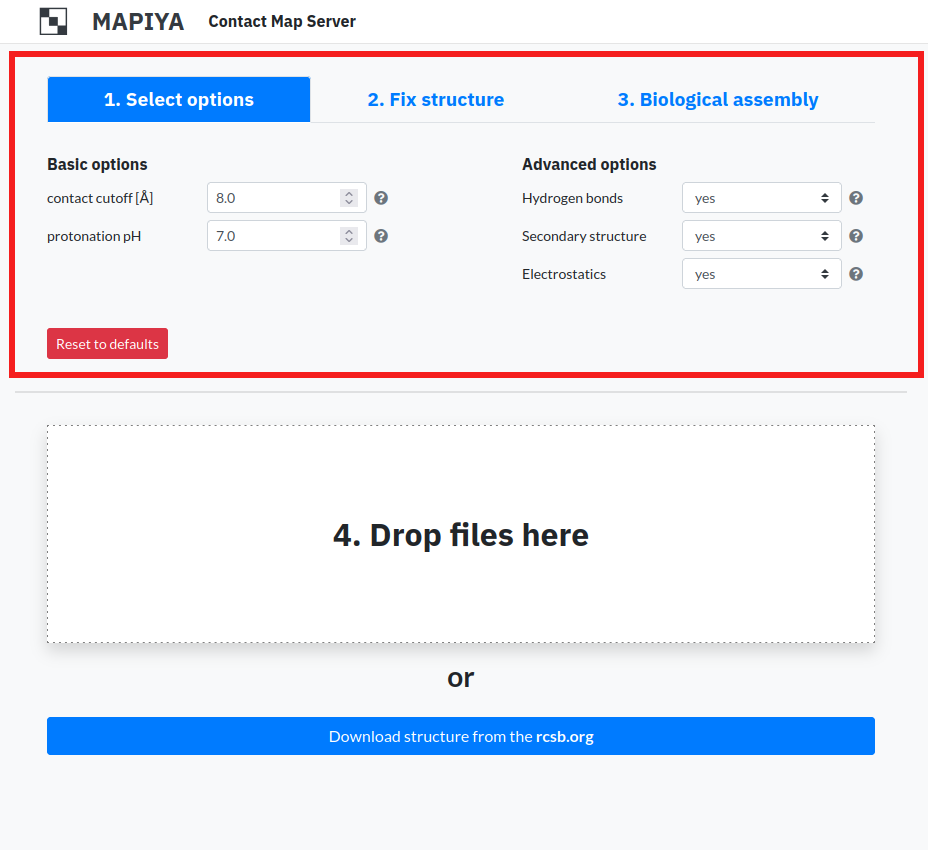
The main Mapiya page allows providing input structure along with several options.
1.1. Select options
The first panel “Select options” contains the following basic options:
- Contact cutoff – User sets the value for contact cutoff (in angstrom [Å]). The distance between the two closest heavy atoms in two different residues is considered contact if it is below the contact cutoff value. In the project view for a particular file, the user can later change this value and display contact maps for the changed contact cutoff.
- Protonation pH – The user sets the value for pH of the modeled environment. The value can range between 0 and 14. The protonation pH is used to define the environmental conditions for structure repair with PDBFixer (e.g., selecting the protonation state of a residue when adding hydrogens or adding environment) and electrostatic analysis performed with APBS (e.g., calculating electrostatic potential). The value can range between 0 and 14, with the default set up to 7. The protonation pH can be adjusted only before submitting the job to a queue, i.e., before the computationally extensive step of Mapiya’s analyses. If a change of the pH value is needed, the user should create a new Mapiya project.
- Calculate hydrogen bonds – If this option is checked, Mapiya calculates hydrogen bonds using EDHB
(https://github.com/ekraka/EDHB).
Note: The structure has to have hydrogens to calculate hydrogen bonds. - Calculate secondary structure – If his option is checked, Mapiya calculates secondary structure using STRIDE (http://webclu.bio.wzw.tum.de/stride).
- Calculate electrostatics – If this option is checked, Mapiya calculates electrostatics using Adaptive Poisson-Boltzmann Solver (APBS) software (https://github.com/Electrostatics/VR).
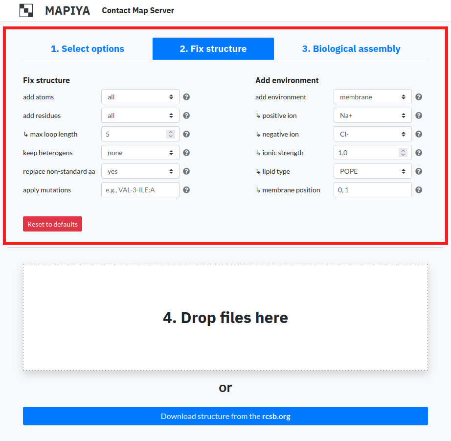
1.2. Fix structure
The second "Fix structure" panel contains input options for PDBFixer (https://github.com/openmm/pdbfixer). PDBFixer is an encapsulated application that makes it easy to use the functionality provided by OpenMM, a comprehensive molecular dynamics simulation toolkit. We chose this software because of its
- (i) transferability,
- (ii) extensibility,
- (iii) ability to efficiently use computing power (CPU and GPU),
- (iv) flexible adaptation for various modeling tools (e.g., Amber, CHARMM, Gromacs, Desmond).
The options available in this section are:- Add atoms – This option enables users to add missing atoms to the structure. The available options are: all, heavy, standard, terminal, hydrogen and none. The default option is all.
- Add residues – This option enables users to add missing residues to the structure. If the residues are to be added, the user has to specify the maximal length of inserted loops. The available options are: all, internal, terminal, none. The default option is all.
- Keep heterogens – This option enables users to keep heterogeneous atoms from being removed. The available options for heterogens to be kept are: all, water, none. The default option is none.
- Replace non-standard aa – This option enables users to replace all non-standard amino acids in the structure for their standard equivalents. The default option is yes.
- Apply mutations – This option enables users to apply mutations in the structure. The input is in form: three-letter amino acid code for an original residue - index of a residue that is being replaced - three-letter amino acid code for a mutated residue : protein chain id. For example VAL-7-ILE:A will mutate valine 7 into isoleucine in chain A. The multiple mutations may be entered, separted by comma.
- Add environment – This option enables users to add an environment to a modeled project. The available options are: none, solvent, membrane.
To add solvent user has to specify:- type of positive ion,
- type of negative ion,
- ionic strength,
- water box – unit cell, max size, or custom.
- type of positive ion,
- type of negative ion,
- ionic strength,
- lipid type,
- membrane position (the position along the Z axis at which the center of the membrane will be located) and minimum padding (the minimum acceptable distance between the protein and the edges of the periodic box).
1.3. Biological assembly
For structures solved by X-ray diffraction, the PDB formatted files contain only the asymmetric unit and this may or may not be the same as the biologically relevant structure. An asymmetric unit may contain: a) one biological assembly, b) a fraction of the biological assembly or c) more than one biological assembly. Mapiya allows users to generate biological assemblies. On the main page, under the third tab, users can select the option Create separate projects for each biological assembly.
The ‘REMARK 300’ in the PDB file is read to determine the number of biological assemblies that need to be generated for the PDB file submitted by the user. An example of REMARK 300 from the PDB ID 3HL2 is provided below: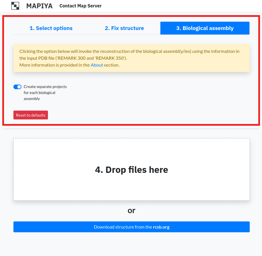
REMARK 300 BIOMOLECULE: 1, 2
The ‘REMARK 350’ from the PDB file is read to determine the chains from each biological assembly and to identify the corresponding ‘BIOMT’ matrices. The BIOMT matrices are transformation matrices, both rotation and translation, when applied we can generate the full assembly. An example of REMARK 350 from the PDB ID 3HL2 is shown below:
REMARK 300 SEE REMARK 350 FOR THE AUTHOR PROVIDED AND/OR PROGRAM
REMARK 300 GENERATED ASSEMBLY INFORMATION FOR THE STRUCTURE IN
REMARK 300 THIS ENTRY. THE REMARK MAY ALSO PROVIDE INFORMATION ON
REMARK 300 BURIED SURFACE AREA.
REMARK 300 REMARK: THE PHYSIOLOGICALLY ACTIVE TETRAMERIC ASSEMBLY CAN BE
REMARK 300 RECONSTRUCTED BY APPLYING THE FOLLOWING SYMMETRY OPERATION ONTO THE
REMARK 300 CHAINS A AND B, AND THE CONFORMER A OF THE CHAIN E: X, X-Y, -Z (0 -
REMARK 300 1 0). SIMILARLY, THE PHYSIOLOGIC TETRAMER CAN BE BUILT BY APPLYING
REMARK 300 THE SYMMETRY OPERATION ONTO THE CHAINS C AND D, AND THE CONFORMER B
REMARK 300 OF THE CHAIN E: -X+Y, Y, -Z+1/3 (0 0 0).REMARK 350
Using these remarks the biological assemblies for the molecule are generated. In the example above there are two biological assemblies generated. For each of the assemblies, a new project is created by Mapiya. Here in this example human SepSecS in complex with non acylated tRNASec (PDB ID: 3HL2), the asymmetric unit consists of four protein chains (chains A, B, C, D) and one RNA chain (chain E) as seen in the figure below. The asymmetric unit contains crystallographic contacts which do not have biological significance.
REMARK 350 COORDINATES FOR A COMPLETE MULTIMER REPRESENTING THE KNOWN
REMARK 350 BIOLOGICALLY SIGNIFICANT OLIGOMERIZATION STATE OF THE
REMARK 350 MOLECULE CAN BE GENERATED BY APPLYING BIOMT TRANSFORMATIONS
REMARK 350 GIVEN BELOW. BOTH NON-CRYSTALLOGRAPHIC AND
REMARK 350 CRYSTALLOGRAPHIC OPERATIONS ARE GIVEN.
REMARK 350
REMARK 350 BIOMOLECULE: 1
REMARK 350 AUTHOR DETERMINED BIOLOGICAL UNIT: PENTAMERIC
REMARK 350 APPLY THE FOLLOWING TO CHAINS: A, B
REMARK 350 BIOMT1 1 0.500000 0.866025 0.000000 83.40900
REMARK 350 BIOMT2 1 0.866025 -0.500000 0.000000 -144.46863
REMARK 350 BIOMT3 1 0.000000 0.000000 -1.000000 0.00000
REMARK 350 APPLY THE FOLLOWING TO CHAINS: A, B, E
REMARK 350 BIOMT1 2 1.000000 0.000000 0.000000 0.00000
REMARK 350 BIOMT2 2 0.000000 1.000000 0.000000 0.00000
REMARK 350 BIOMT3 2 0.000000 0.000000 1.000000 0.00000
REMARK 350
REMARK 350 BIOMOLECULE: 2
REMARK 350 AUTHOR DETERMINED BIOLOGICAL UNIT: PENTAMERIC
REMARK 350 APPLY THE FOLLOWING TO CHAINS: C, D
REMARK 350 BIOMT1 1 -1.000000 0.000000 0.000000 0.00000
REMARK 350 BIOMT2 1 0.000000 1.000000 0.000000 0.00000
REMARK 350 BIOMT3 1 0.000000 0.000000 -1.000000 78.77400
REMARK 350 APPLY THE FOLLOWING TO CHAINS: C, D, E
REMARK 350 BIOMT1 2 1.000000 0.000000 0.000000 0.00000
REMARK 350 BIOMT2 2 0.000000 1.000000 0.000000 0.00000
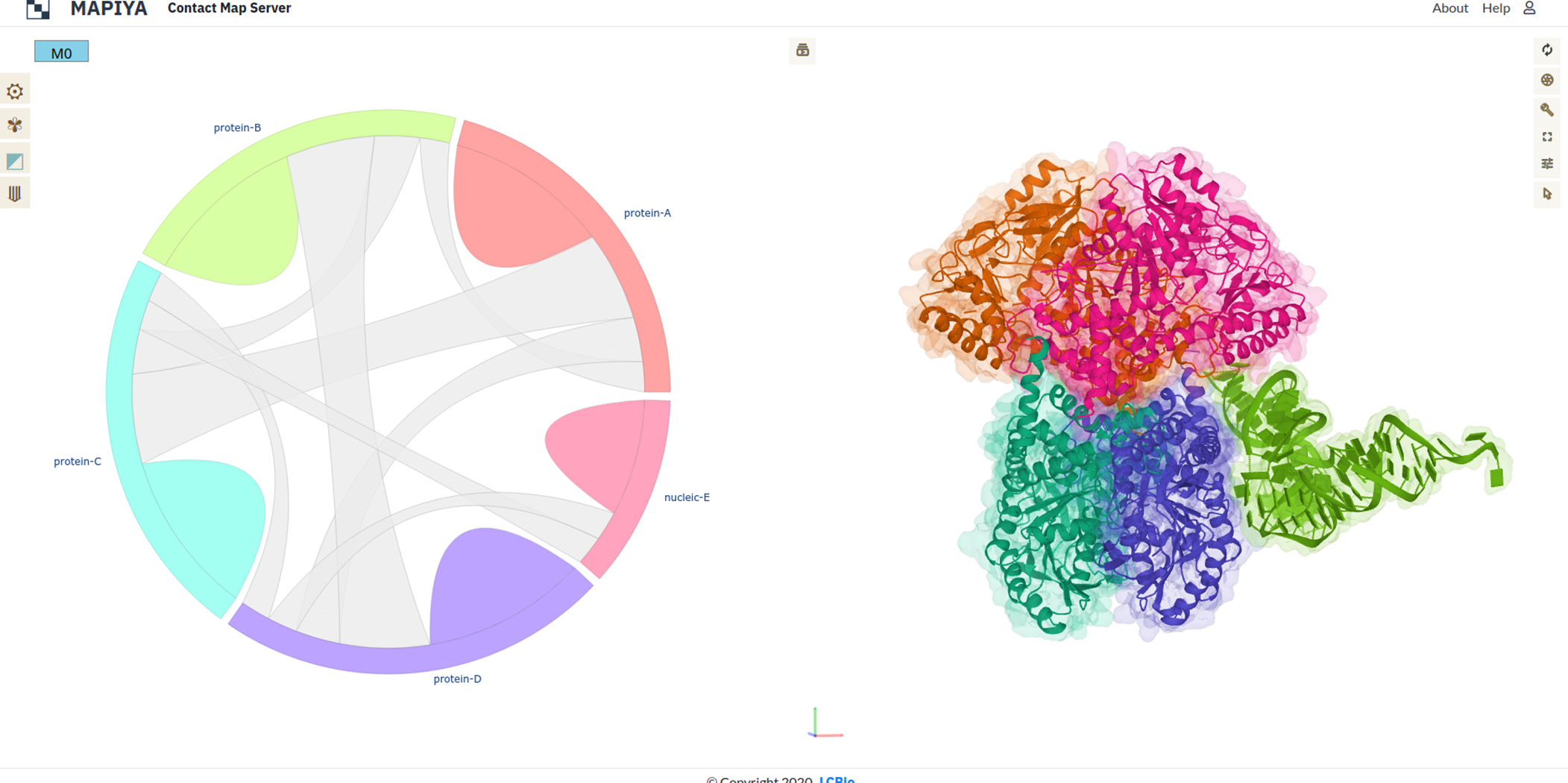
REMARK 350 BIOMT3 2 0.000000 0.000000 1.000000 0.00000Using the REMARKS 300 and 350, we can generate two biological assemblies. The first assembly consists of chains A, B, E from the asymmetric unit without modifications and chains C and D which are generated by applying the BIOMT transformation matrix to original chains A and B (see figure below).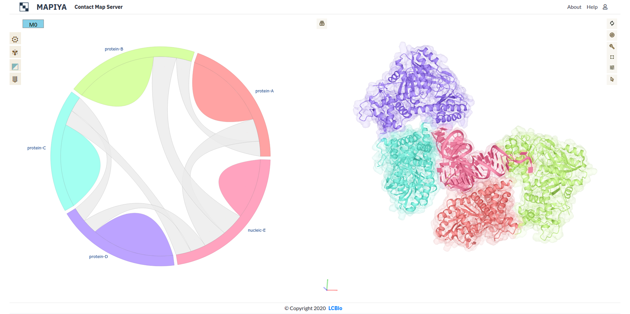 Similarly, the second assembly consists of chains C, D, and E from the asymmetric unit without applying modifications, and chains A and B which are generated by applying the BIOMT transformation matrix to chains C and D from the asymmetric unit (see figure below).
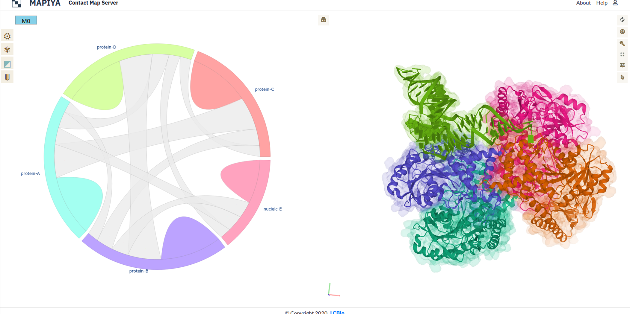
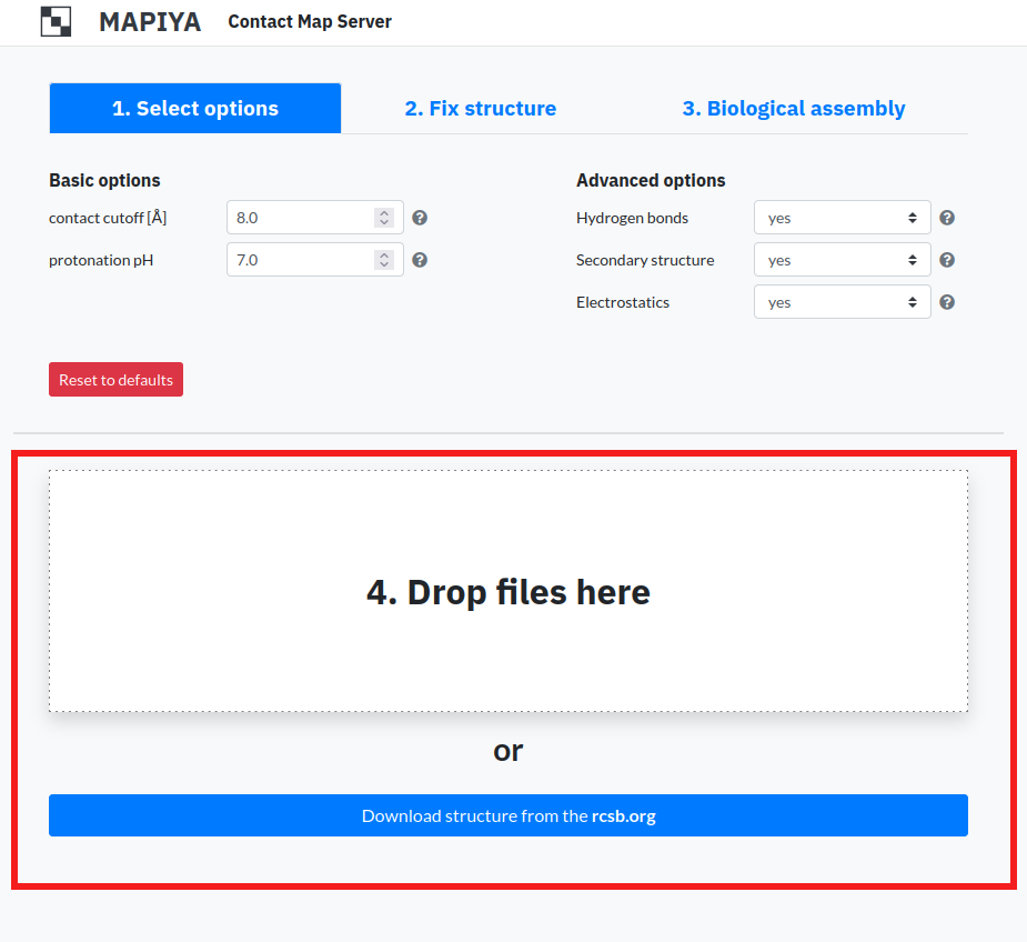
1.4. Download structure files
In order to submit a project for calculation, the user either has to either submit a PDB file from disk or enter PDB code to download the file from the RCSB database. The PDB file cannot exceed 50 models. There are two options to submit project:
- Drop files here – In order to submit a file the user has to drag and drop a file located locally on a disk.
- Download structures from the rcsb.org – In order to submit a file the user has to enter PDB code. Mapiya downloads the structure from the RCSB database and submits the project for a calculation.
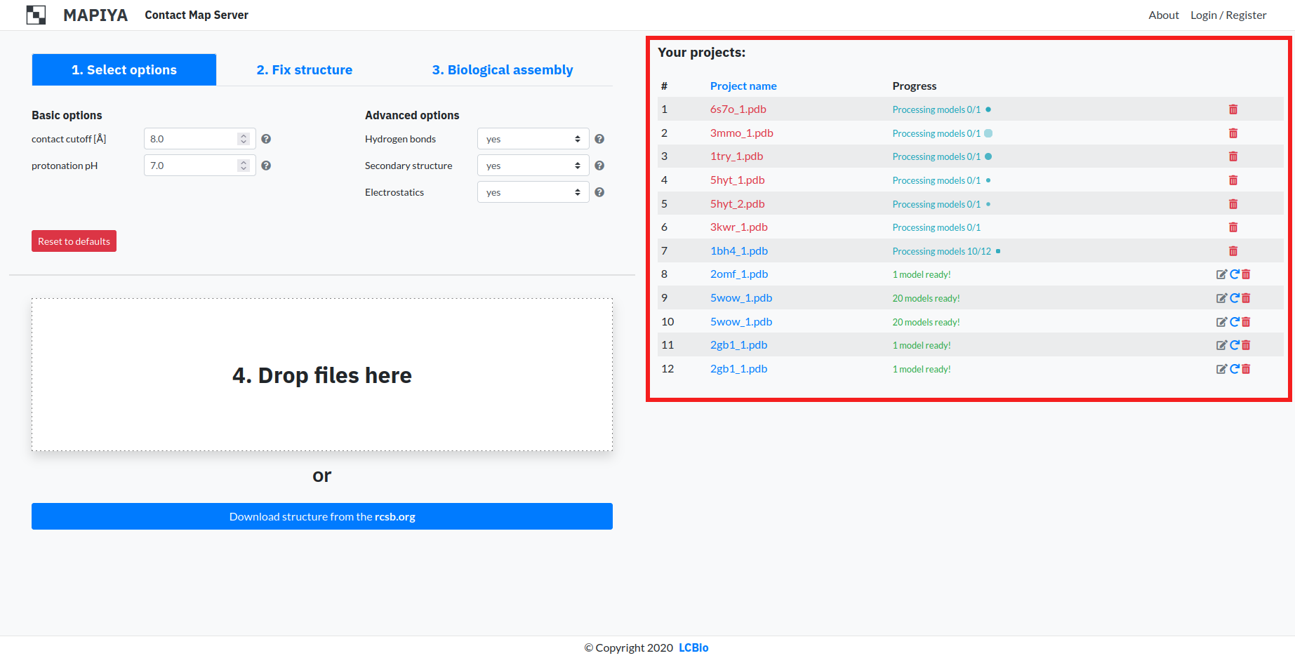
1.5. Project list
The list consists of every project submitted or calculated. Every entry consists of this information:
- Project name – This column displays the name of the project. After calculation finishes, clicking on the name takes the user to the project view for that submitted file. It can be changed by clicking 'Rename project' button on the right side of table.
- Progress – This column displays the state of a particular project. When the caption turns green, it means the project has finished calculating.
- Rename project – This button enables users to rename projects.
- Resubmit – This button appears after the project has finished calculating. It enables users to recalculate projects i.e. after changing options.
- Delete – This button enables the user to delete the project from the database and Project list.
2. Diagram view
When preliminary calculations (distance matrix and structural analysis) for a given project are ready, Mapiya
loads the interaction diagram (see Figure below). In this view, Mapiya draws connections between molecules in
a complex (objects located on the perimeter of a circle) with a ribbon thickness proportional to the number
of contacts. The different chains of the macromolecule have distinct colors with correspondence between a
circular diagram on the left side and the Molstar viewer on the right. Users can switch to the map view using
options from the menu or interactively by clicking on the ribbon of interest. Selecting the ‘intramolecular’
option or a bulge in the discrete color will load the internal contact map for the matching chain. Selecting
the ‘intermolecular’ option or one of the gray ribbons will load the map of the contact interface between two
molecules. When the submitted PDB has multiple models, the user can display the results for the particular
model by clicking on the corresponding button at the top of the screen.
The Figure below shows an example interaction diagram view for the complex between trp RNA-binding attenuation
protein (TRAP) and 55-mer single-stranded RNA (PDB ID: 1C9S). The diagram shows that each of the eleven protein
chains in the assembly interacts with two adjacent protein chains and the RNA.
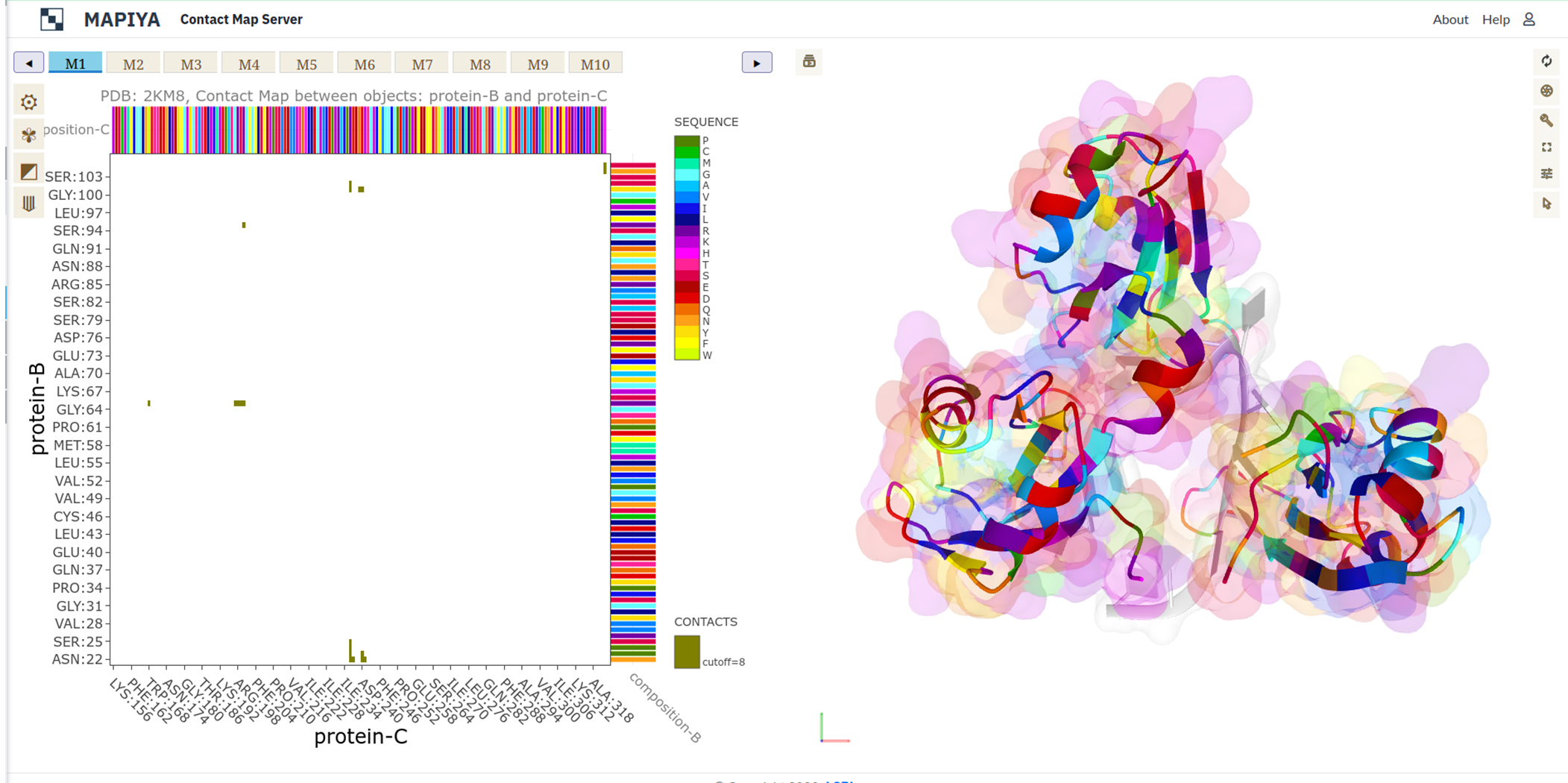
 Another example below presents RNA recognition motif (RRM) domains of the cleavage factor IA and Hrp1 proteins,
and a 14-mer RNA (PDB ID: 2KM8). In this example, there are ten conformers available in the PDB file and we can
navigate between them in Mapiya by clicking on the panel with model numbers (see Figure below, highlighted with a red box).
Another example below presents RNA recognition motif (RRM) domains of the cleavage factor IA and Hrp1 proteins,
and a 14-mer RNA (PDB ID: 2KM8). In this example, there are ten conformers available in the PDB file and we can
navigate between them in Mapiya by clicking on the panel with model numbers (see Figure below, highlighted with a red box).
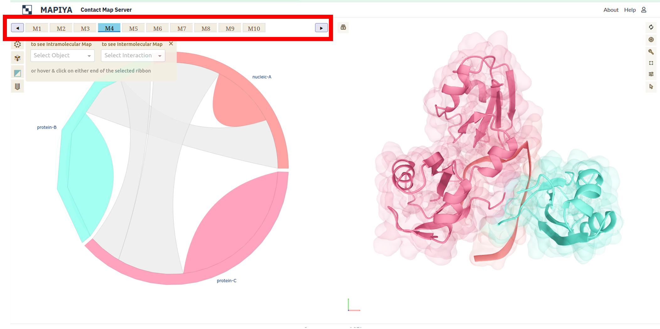 Each chain from the selected model is colored with unique and distinct colors in the interaction diagram. The
contact between the residues in different chains are shown as connections in the interaction diagram (on the left).
On the right side, the selected model is rendered in three-dimensions in the Molstar viewer and the chains are colored
in the same way as in the diagram. By default, Mapiya shows two representations of the molecule in 3D,
using the cartoon and the Gaussian surface representation. The user can add additional representations supported by
Molstar viewer. A detailed tutorial on the use of Molstar viewer and the different options available to the users
can be found at: Common actions - Molstar Viewer Documentation
and RCSB Molstar - getting started.
Each chain from the selected model is colored with unique and distinct colors in the interaction diagram. The
contact between the residues in different chains are shown as connections in the interaction diagram (on the left).
On the right side, the selected model is rendered in three-dimensions in the Molstar viewer and the chains are colored
in the same way as in the diagram. By default, Mapiya shows two representations of the molecule in 3D,
using the cartoon and the Gaussian surface representation. The user can add additional representations supported by
Molstar viewer. A detailed tutorial on the use of Molstar viewer and the different options available to the users
can be found at: Common actions - Molstar Viewer Documentation
and RCSB Molstar - getting started.
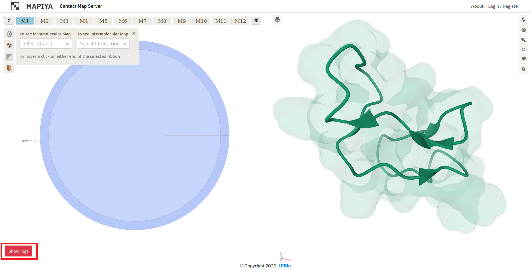
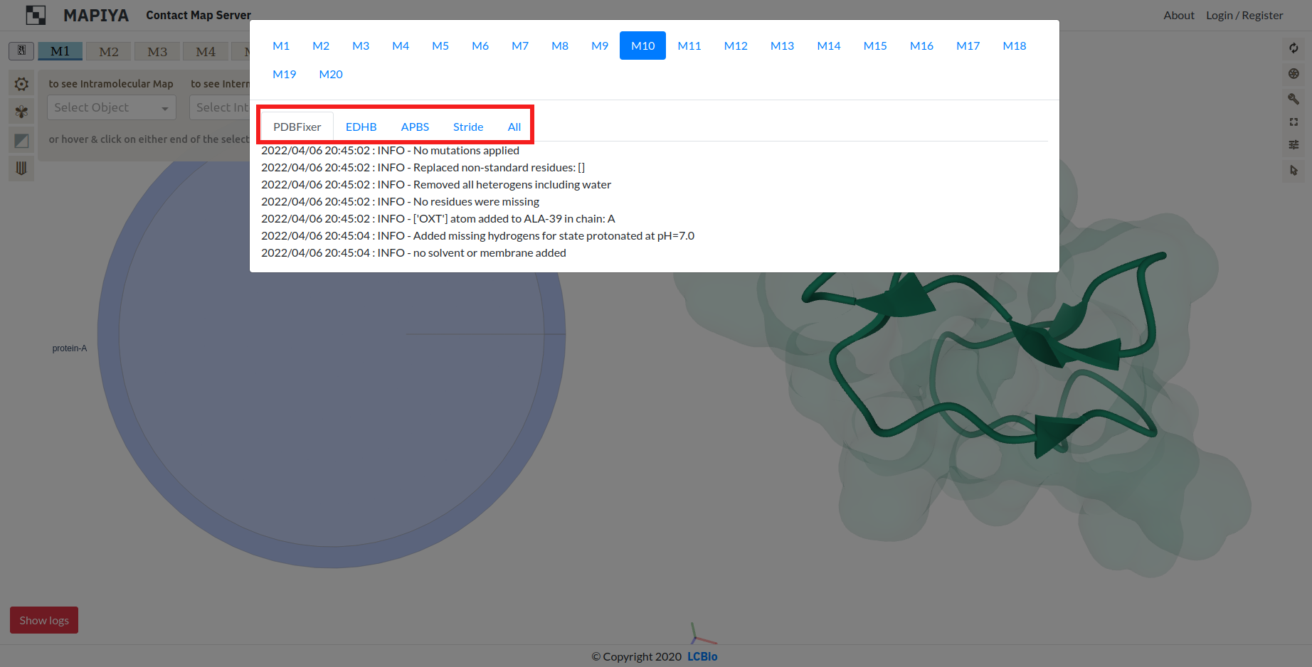
There is a red 'Show logs' button in the lower left corner. Logs can provide inside to why some calculations have not returned expected results. The users can display logs from calculations done by external software by clicking on the button.
 The logs are divided in five categories:
- PDBFixer
- EDHB
- APBS
- Stride
- All
3. Map
To display the MapView, the user has to choose either Object (Intramolecular Map) or Interaction (Intermolecular
Map) from the list. The two types of maps are:
- The intramolecular map, shows the internal contacts of the selected object. These contacts stabilize the
secondary structure and topology of a single domain.
- The intermolecular map, shows the spatial contacts between two selected objects. These contacts
define binding interfaces, stabilize the quaternary structure, and are important for function.
3.1. Basic options
The MapView of the Mapiya web server consists of an interactive heatmap chart. The graph has three available display modes:
- DM, Distance Map, where the points are colored with a continuous color scale according to the distance between corresponding residue pairs,
- CM, Contact Map, where the points are colored with a discrete (or smooth) color scale according to the identified spatial contacts,
- CM | DM, where the chart is split into two triangles (this mode is available only for Intramolecular maps).
Multiple Color scales are available for user convenience. Discrete (binary) color scales for CM mode can be easily smoothed to continuous scales, making it easy to distinguish the strength of contacts by distance of interacting residues. In DM and CM | DM mode, the color scale can also be reversed.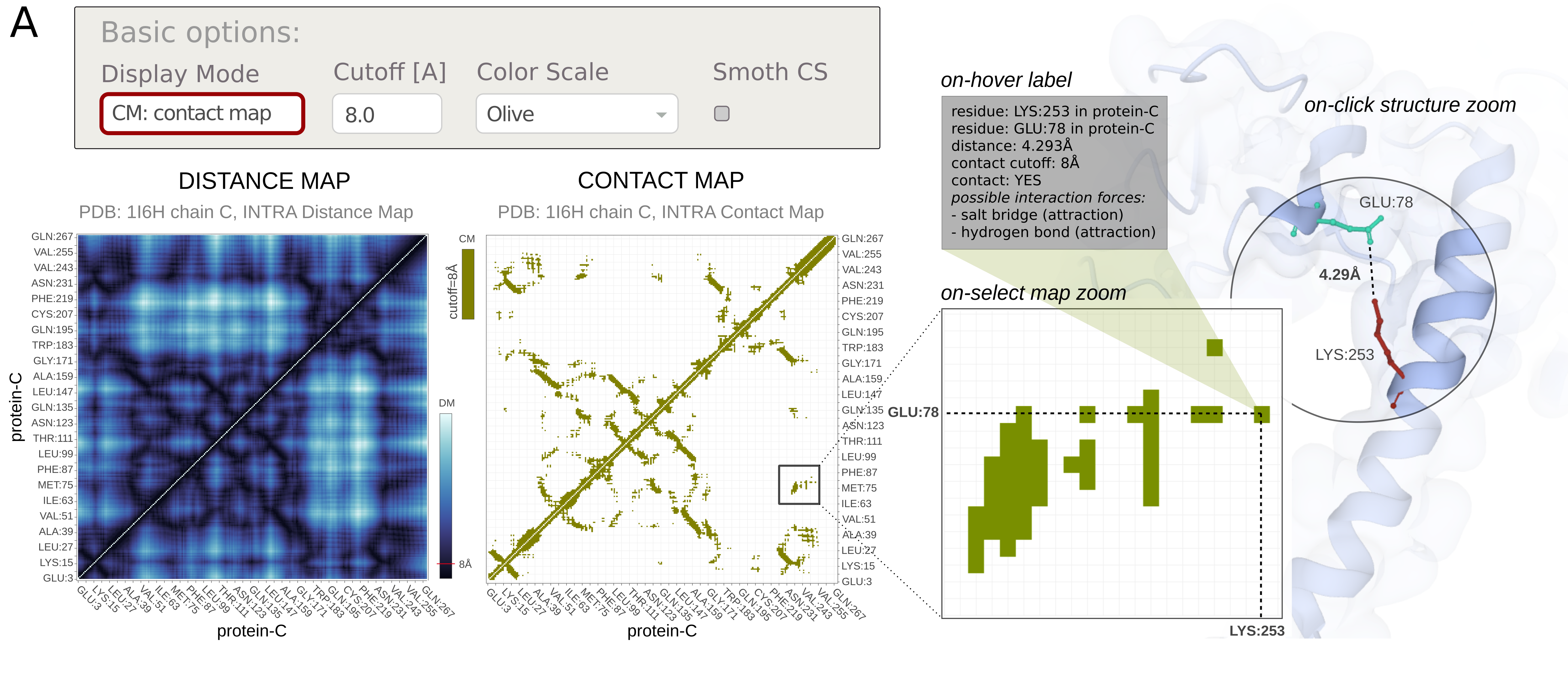
There is also an option to change the distance Cutoff for contacts. After the contact cutoff value has been changed, the map dynamically changes accordingly.
The last option enables users to choose Interactive structure coloring. The structure can be colored by default (the option none), by contacts, or by 1D features (the 1D features must be selected in Displaying 1D data section below). The default option is none.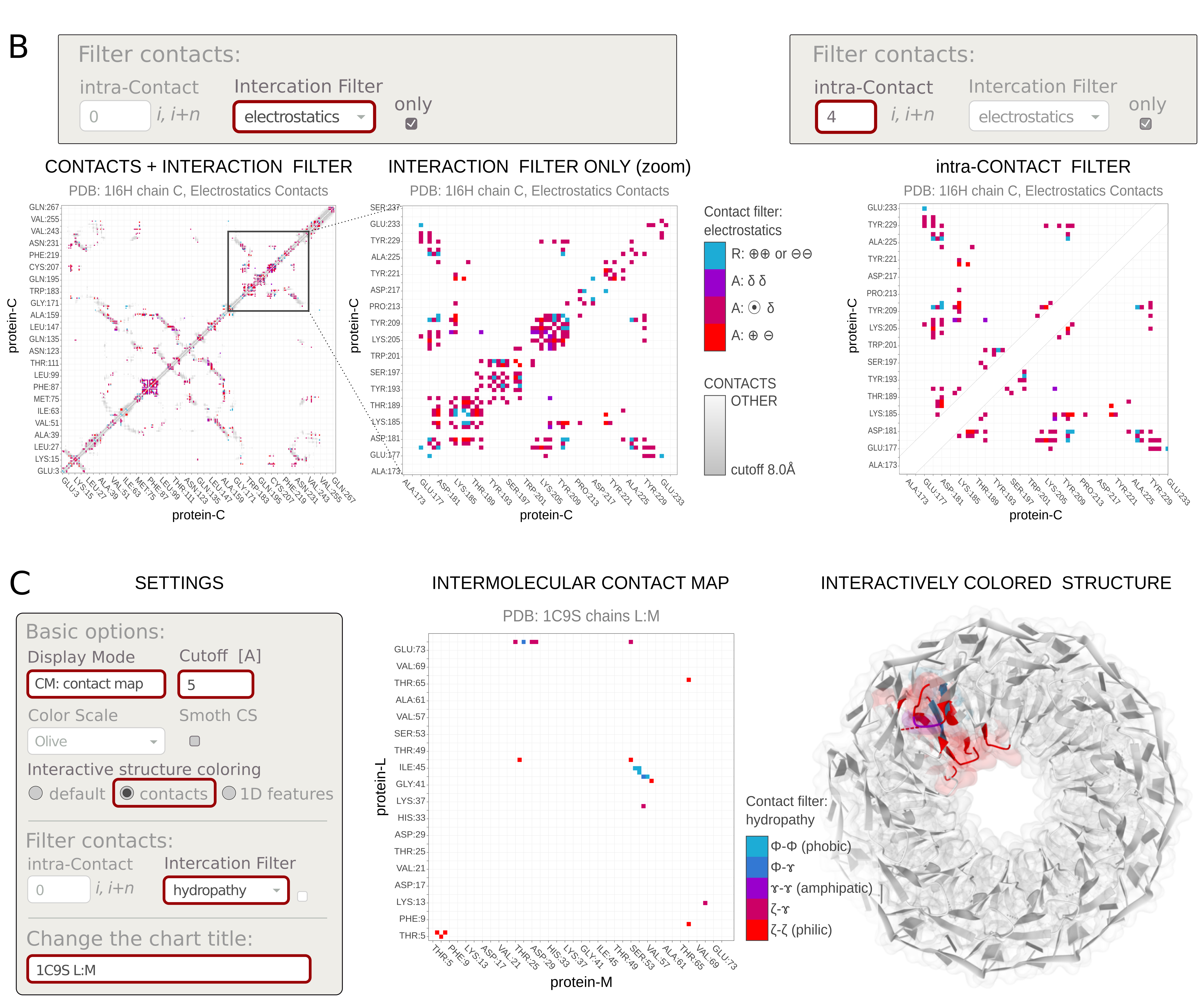
3.2 Contact filters
Using Filter contacts options, you can cross-select contacts by properties or screen-out them by sequential neighborhood. The user can highlight the protein-protein contacts stabilized by the selected interaction type. This facilitates your discovery of the nature of the interaction.
Specifically, the Interaction filter selects contacts by various physicochemical properties of interacting residues. Note: Some contacts can be multivalent (e.g., have both charge and π-electrons) and can be displayed for several force types (e.g., electrostatics and π-stacking). Each option in the Interaction filter has its own tooltip.The available options include: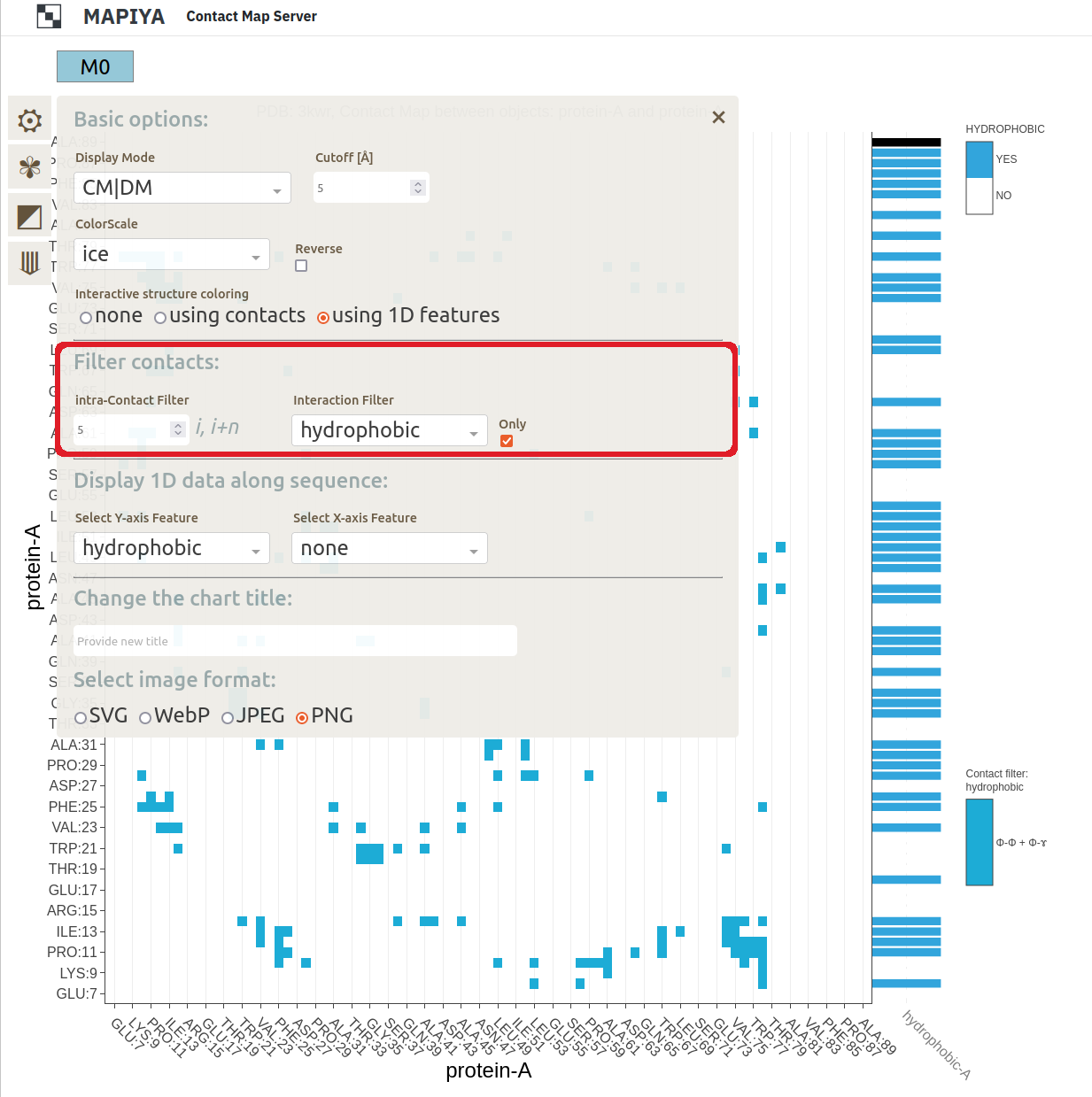
- hydropathy: hydrophobic, hydrophilic, amphipathic
The hydropathy shows the hydrophobic (lacking affinity for water), amphipathic (having both polar-water-soluble and nonpolar-not-water-soluble regions), and hydrophilic (attracted to water) tendencies of the protein sequence.
The hydrophobic (Φ) amino acids are: Gly, Ala, Leu, Ile, Val, Pro, Phe.
The amphipathic (ɤ) amino acids are: Trp, Tyr, Met, Lys.
The hydrophilic (ζ) amino acids are: Arg, Asn, Asp, Gln, Glu, His, Ser, Thr, Cys. - electrostatics: ion-ion, ion-dipole, dipole-dipole
Electrostatics describes the interactions between charges. There is an attractive (A) force between a positive ⊕ and a negative ⊖ charge, while two charges of the same sign repel (R) each other. Point charges (monopoles) such as ions ⦿ , can also interact electrostatically with dipoles (e.g polar groups, δ) and cause temporary charge shifts (induced dipoles) in neutral groups.
Positively charged amino acids, ⊕ are: Arg, Lys, His.
Negatively charged amino acids, ⊖ are: Glu, Asp.
Polar amino acids, δ are: Ser, Thr, Tyr, Gln, Asn, Cys, Met. - π-electron stacking: π-π, cation-π, anion-π, dipole-π
π–π stacking is an attractive, noncovalent interaction between aromatic rings, ⌬ , and/or other π–electron-containing systems. Ion–π interaction is a noncovalent attractive interaction between the electron-rich π-system (e.g. aromatic ring ⌬ or other π-bond) and an adjacent ion, i.e., cation ⊕ or anion ⊖. The ion-π interactions are orientation-dependent. The two most stable conformations are the parallel displaced and T-shaped.The stacking is also possible between the π–electron-containing system and polar group or even C-H orbital.
The aromatic amino acids, ⌬ are: Phe, Tyr, trp, His.
The other systems with π–bond are: Arg, Asn, Asp, Gln, Glu, Gly*. - hydrogen bonds (calculated using EDHB)
A hydrogen bond is a special type of dipole-dipole attraction, involving a hydrogen atom located between a pair of highly electronegative atoms (having a high affinity for electrons). Hydrogen bonds are calculated using EDHB. If the option is disabled, the process was unsuccessful.
Amino acids that can be proton donors: Arg, Asn, Gln, His, Ser, Thr, Tyr, Trp, Cys, Lys.
Amino acids that can be proton acceptors: Asn, Asp, Gln, Glu, His, Ser, Thr, Tyr.
Additionally, the Intra-contact filter removes local contacts between residues neighboring along the sequence. As a result, the points along the diagonal of the intramolecular (internal) contact map are dropped. The filter takes an integer n, which defines the number of amino acids (i, i+1, ..., i+n) along the sequence, for which contacts are excluded.
There is an option to display filtered contacts Only. This removes the other contacts from the background of the plot.- hydropathy: hydrophobic, hydrophilic, amphipathic
3.3. Displaying 1D data
Using Display 1D data options, you can add various one-dimensional features along the objects' sequence. The residue-resolution bar-chart will be displayed on the right side parallel to the Y-, or on the top side parallel to the X-axis. Note: Some contacts can be multivalent (e.g., have both charge and π-electrons) thus such additional sequence- and structure-dependent data facilitate the comprehensive analysis of interactions contributions.
The available options include:- various physicochemical properties,
- amino acid composition,
- secondary structure, calculated using STRIDE
- solvent accessibility, calculated using STRIDE
- Shannon entropy calculated on-the-fly
- hydrogen bond donor/acceptor,
- and more...
Examples are presented in the Figure below.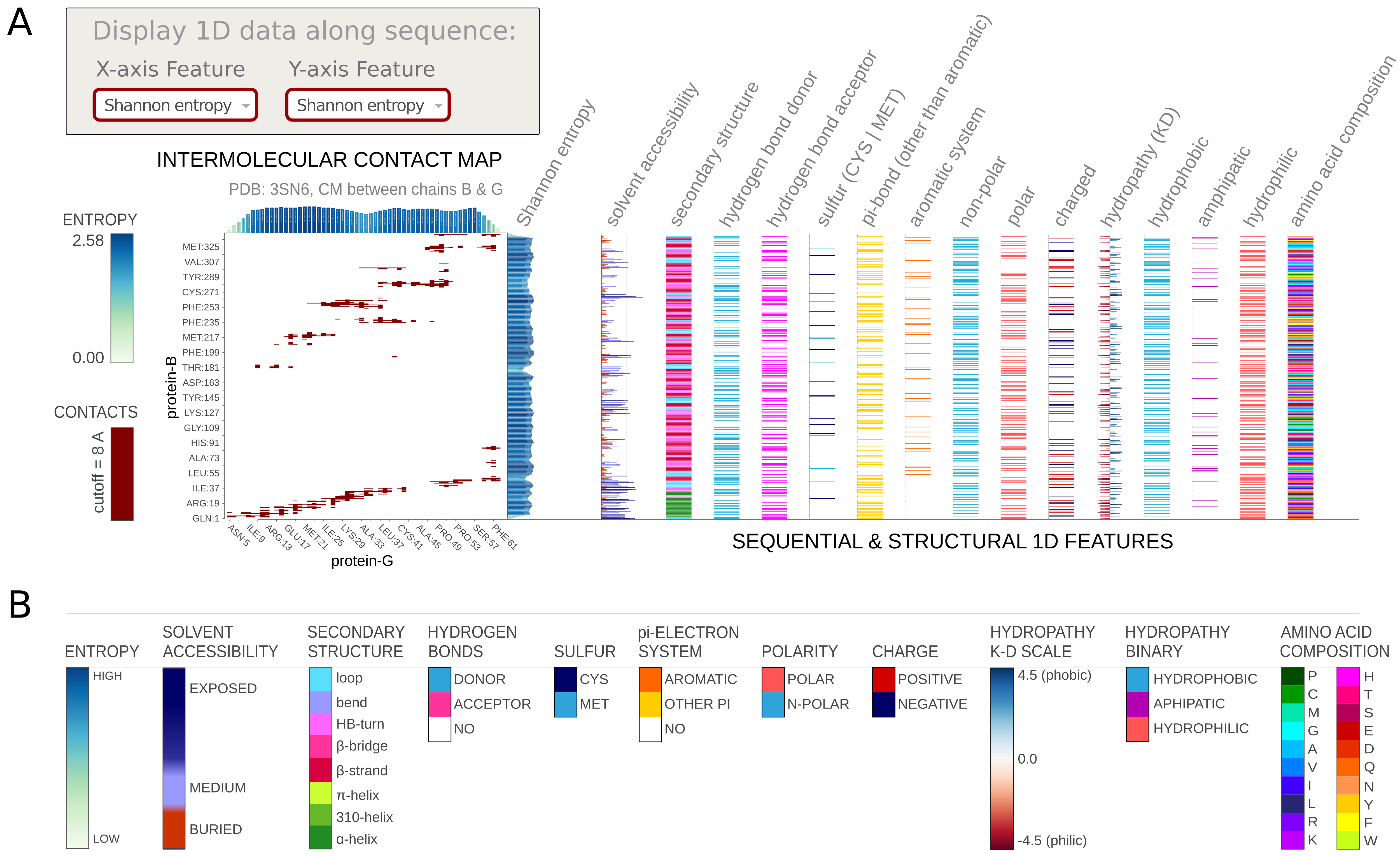
3.4. Generating map images
The last section enables users to change some minor options of generating map images. In the first option - Change the chart title, the user can enter a customized title that will display above the chart. The second option - Select image format, provides the generated map image in either vector (SVG) or raster (JPEG, PNG) graphics format.
3.5. Interaction of Maps with Molstar molecular visualization
In the map view, the user can select a particular contact between two residues by clicking any points on the map loaded on the left half. When a point is clicked on the map, the corresponding two residues are zoomed in and highlighted in the Molstar viewer. Here we illustrate this with an example of ARG-198 in the Hrp1 protein (Chain C) and ARG-65 (Chain B) in the cleavage factor IA. The two residues are at a distance of 4.654 Å and the distance cutoff is 8 Å. By design, the users are also allowed to click on points, which are not within the distance cutoff, and the corresponding residues will be highlighted on the Molstar viewer.
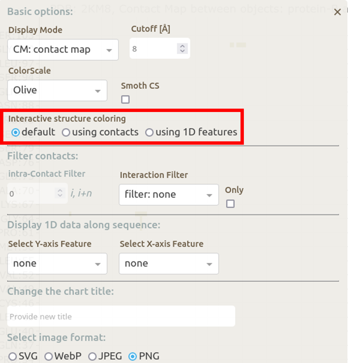 In the basic menu available in the map view, Mapiya provides three options under the Interactive structure coloring option to provide interactivity with the Molstar viewer: default, using contacts and using 1D features. When the map view is loaded, by default, Mapiya uses default as the color choice, which retains the colors displayed in the interaction view. Below, we show an example of the default behavior of Mapiya. Here we show two RRM domains in complex with an RNA (PDB ID: 2KM8) in the map view with default coloring. The three chains are coloured same as in the diagram view.
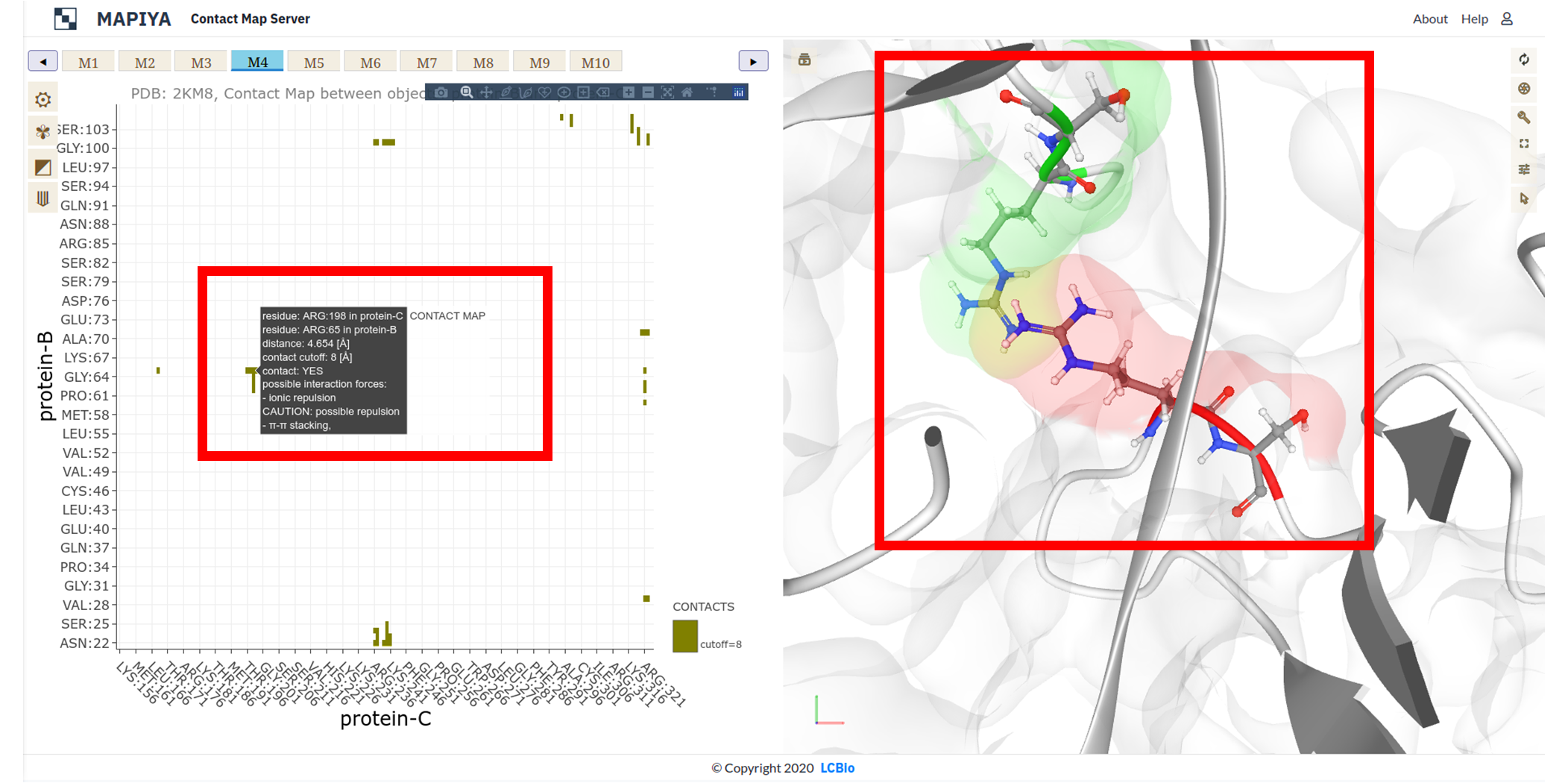 The Using contacts option will only color the residues which are selected based on the cutoff value. All the other residues are grayed out when this option is selected. Below we show the contacts between the two RRM domains at a cutoff distance of 8 Å.
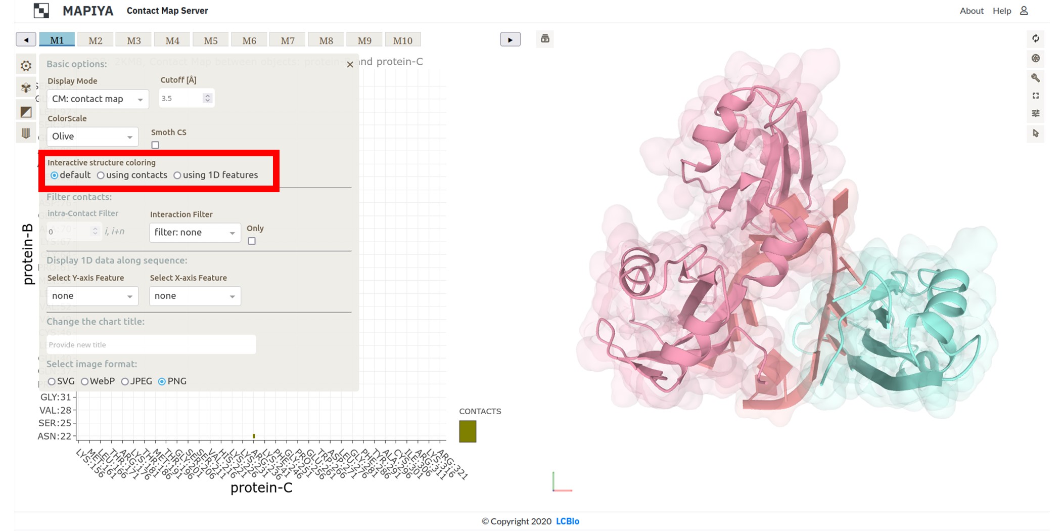 When the Interaction filter option is used to filter the contacts based on structural and physicochemical parameters, this option colors only those residues which are selected by the option. For example, here we show the contacts between the two RRM domains filtered by setting the Interaction filter to Hydropathy and setting the Interactive structure coloring to Using contacts option.
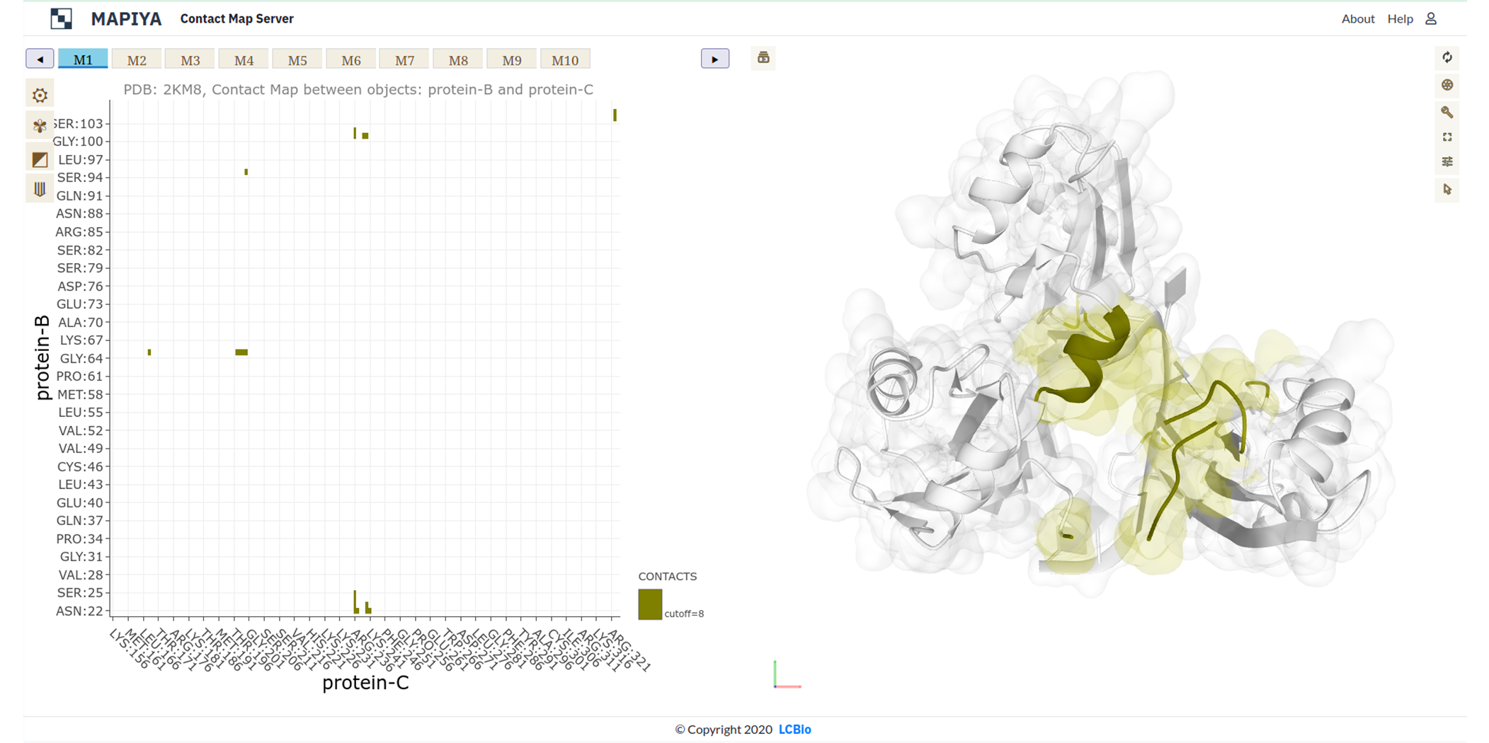 The Using 1D features under the Interactive structure coloring option allows us to color the residues in the molstar viewer based on the option selected in the Display 1D data along the sequence drop-down menus. Here, we illustrate the coloring by using the Composition option selected on both X-axis and Y-axis features options. When the map view is showing intramolecular only one parameter can be used to color the chain.
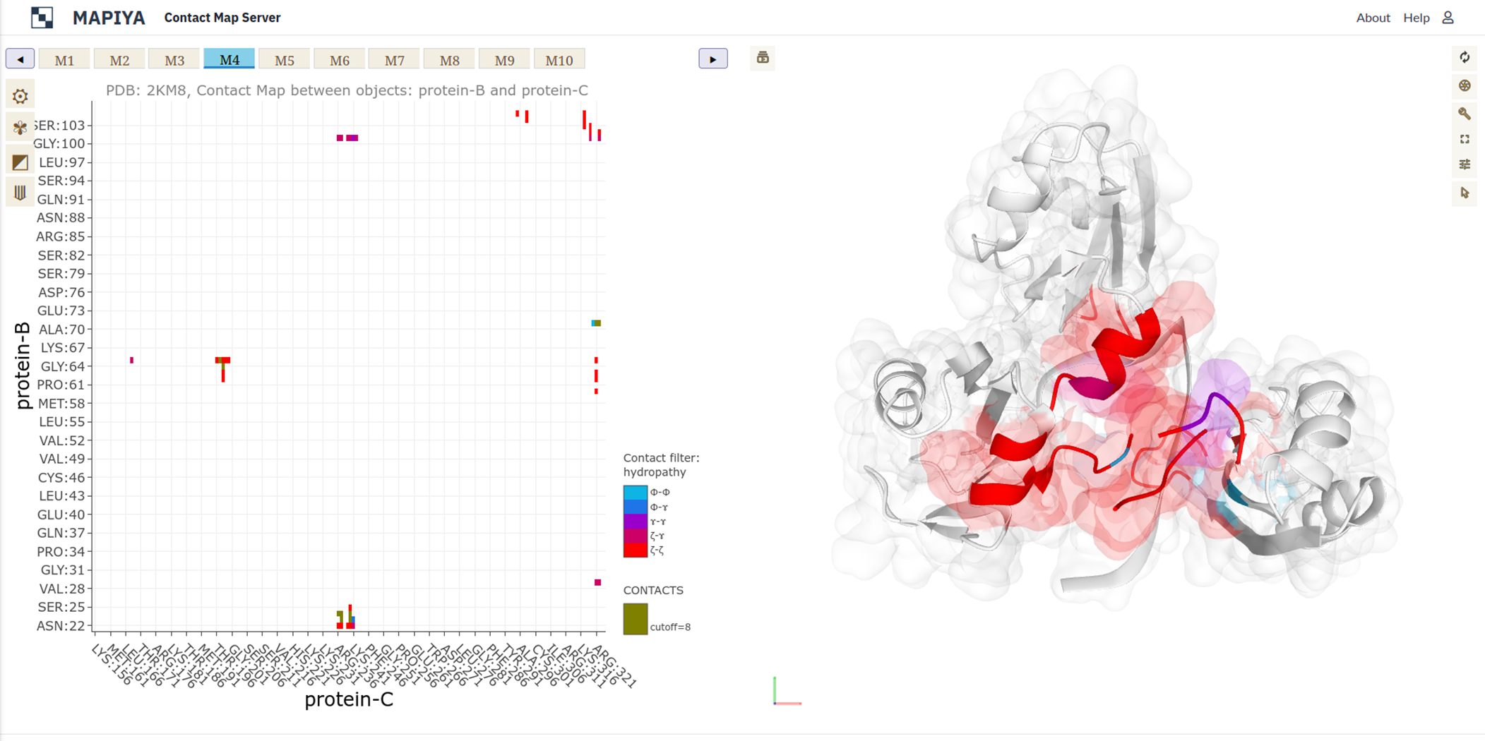
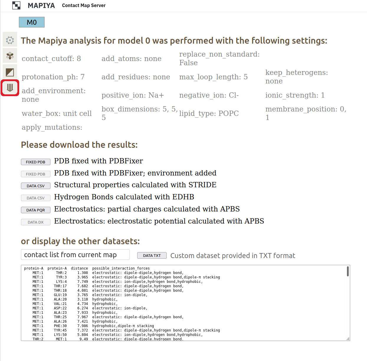
3.6. Downloading data in text format
All the data generated can be downloaded in text format. The location of the download section is shown in the Figure below.
4. Case studies
4.1. Human DNA polymerase
The selected example shows the Mapiya results for a Human DNA polymerase beta complexed with gapped DNA (PDB: 1BPY).
The MapView presents the intermolecular contact map (CM mode) between protein chain A (protein-A, on the X-axis) and DNA strand T (nucleic-T, on the Y-axis). Gray points on the map (left panel) are contacts identified below the distance cutoff of 8.0 A. From these, contacts stabilized by attractive electrostatic interactions (A, marked in red-purple palette) were selected using an Interaction filter. More specifically, we want to see which contacts are bound by the salt bridge. Therefore, we selected Charged from the options available for protein-A (feature for the X-axis) in the Display 1D data section of settings. The bar-chart displayed on the top of the Contact Map shows the pattern of positively (light blue) and negatively (dark blue) charged amino acids along the sequence of protein-A. Since nucleic acid is strongly negatively charged, salt bridges can be formed with positively charged amino acids such as Arg, Lys, and His.
For a better view, we zoomed the interactive graph to the 225-305 fragment along the protein-A sequence. We found an isolated contact between ARG:258 and DG:9 (marked with a black dot).Clicking on a selected point invokes two actions: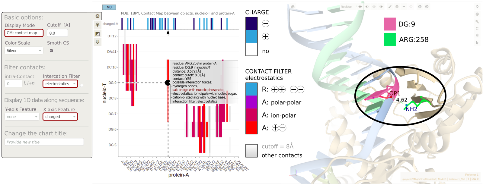
- displays an interactive label with details describing the contact (residues identifiers, distance, possible interaction forces),
- automatically zooms the Mol* Viewer window (right panel) on the residues that are in contact, revealing the atomic details of the interaction.
4.2. TRAP-RNA complex
This case study illustrates some interaction features of the complex between trp RNA-binding attenuation protein (TRAP) and RNA (PDB ID: 1C9S). TRAP is a central regulator in the expression of tryptophan biosynthetic genes (Ref: Gollnick, P. (1994)) and binds to single-stranded RNA (Ref: Babitzke, P., et al. (1994)). The TRAP protein disk consists of eleven identical protein chains bound to a single 55-mer RNA molecule (Ref: Antson, A. A., et al.(1999)). The asymmetric unit of the crystal structure consists of two copies of the TRAP disk with only one bound to RNA. The interaction diagram view generated by Mapiya shows that each protein chain in the assembly interacts with the RNA molecule and two adjacent protein chains (see Figure below).
Each protein chain in the TRAP disk makes contacts with two adjacent protein chains, one on either side and the RNA chain. Here, we highlight the contacts made by chains L and M in the assembly (see figure below). The various options selected to generate the map-view are highlighted with red boxes on the basic settings menu available on the interaction map view.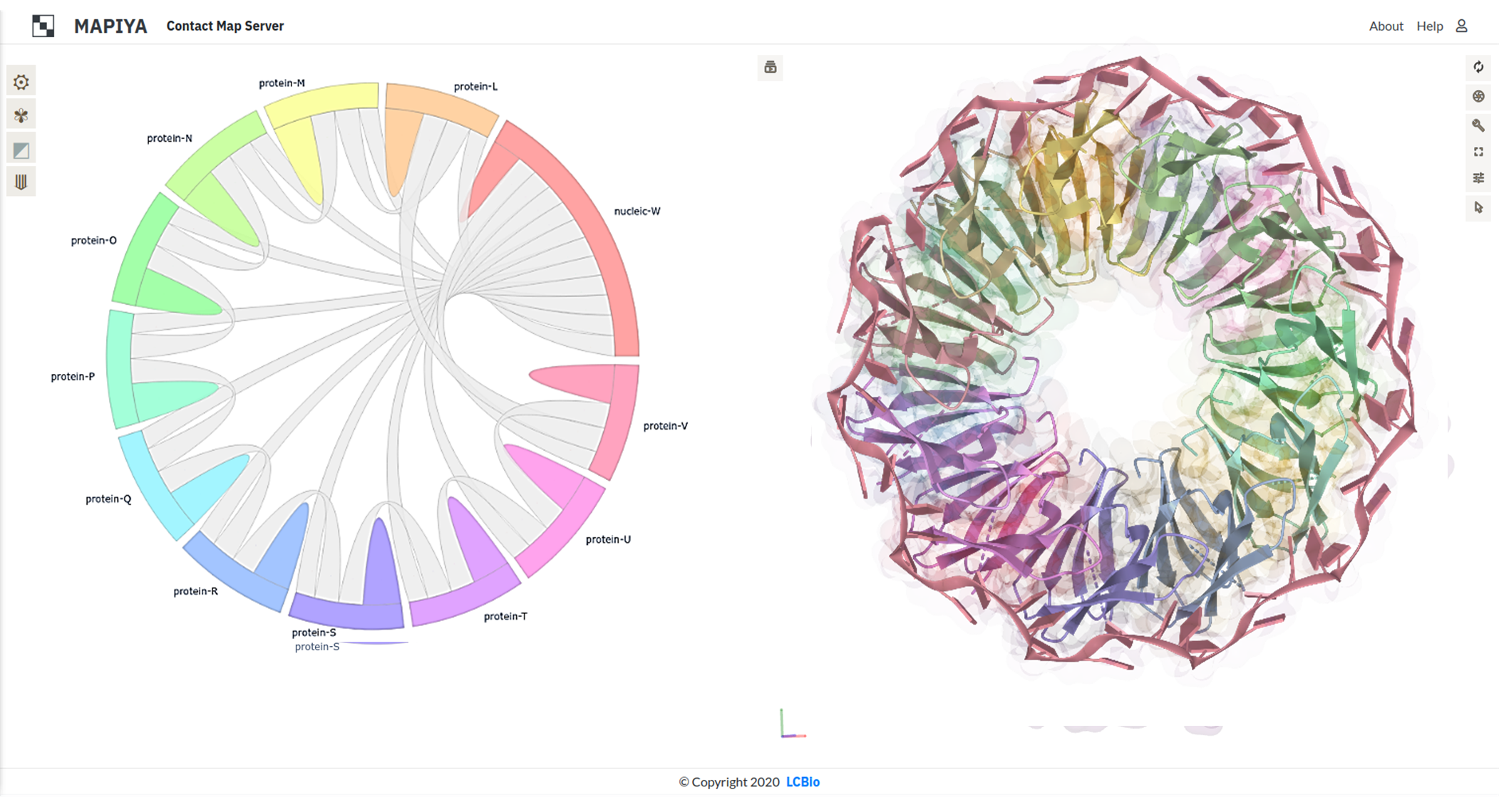 The Interaction map shows contacts between two adjacent protein chains in the TRAP disk, within a distance cutoff 5 Å, filtered with the Hydropathy filter in Mapiya. The interacting residues are colored on the three-dimensional structure rendered using Molstar viewer, with the respective colors from the map view. The color scale used by Mapiya to represent the hydropathy index: hydrophobic (Φ) amino acids (Gly, Ala, Leu, Ile, Val, Pro, Phe), the amphipathic (ɤ) amino acids (Trp, Tyr, Met, Lys), the hydrophilic (ζ) amino acids (Arg, Asn, Asp, Gln, Glu, His, Ser, Thr, Cys), the hydrophobic (Φ) amino acids (Gly, Ala, Leu, Ile, Val, Pro, Phe) and the hydrophilic (ζ) amino acids (Arg, Asn, Asp, Gln, Glu, His, Ser, Thr, Cys).
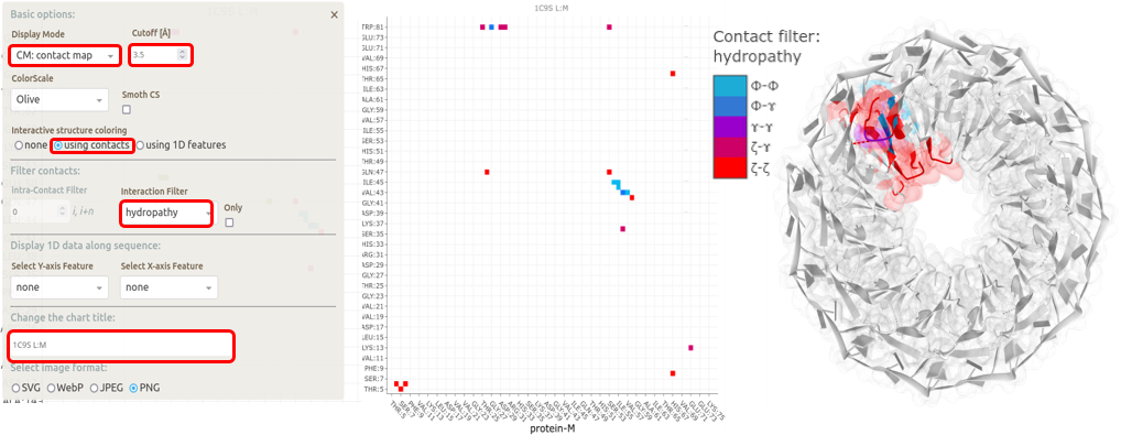
The RNA molecule consists of 5-mer repeats of GAUGA. It has an extended structure in the complex without any base-pairing, with similar three-dimensional structures interacting with the different protein chains. The binding of RNA to TRAP protein is through specific protein-nucleobase interactions with GAG triplets accommodated in a pocket formed by beta-strands. This pocket can be visualized using Mapiya by selecting the 2º structure option available in Display 1D data along the sequence and setting the Interactive structure coloring to Using 1D features (see panels A, B in figure above). The residues that make the contact between the protein and RNA can be highlighted by setting the Interactive structure coloring to Using contacts (see panel C in figure below).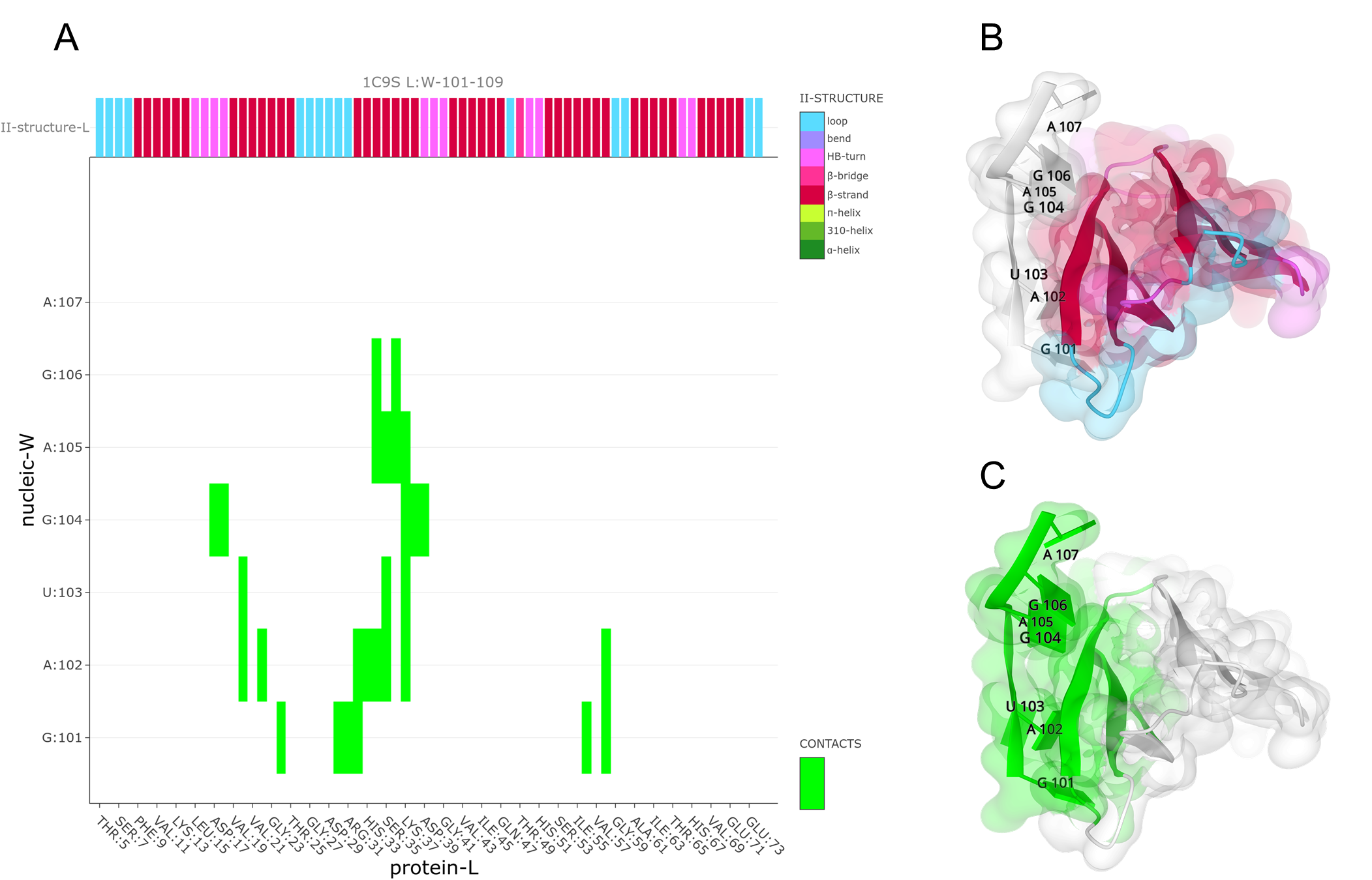
4.3. RNA-dependent polymerase (RdRp)
The use of Mapiya in understanding the structural mechanisms of the biological process can be further illustrated with the example of RNA-dependent RNA polymerase (RdRp) (PDB ID: 6YYT). The active form of RNA-dependent RNA polymerase (RdRp) from SARS-CoV-2 mimics the replication enzyme. In this example, the macromolecular assembly consists of the viral non-structural protein 12 (nsp12), nsp8, and nsp7, along with more than two turns of RNA template-product duplex (Ref: Hillen, H. S., et al. (2020)) (see figure below).
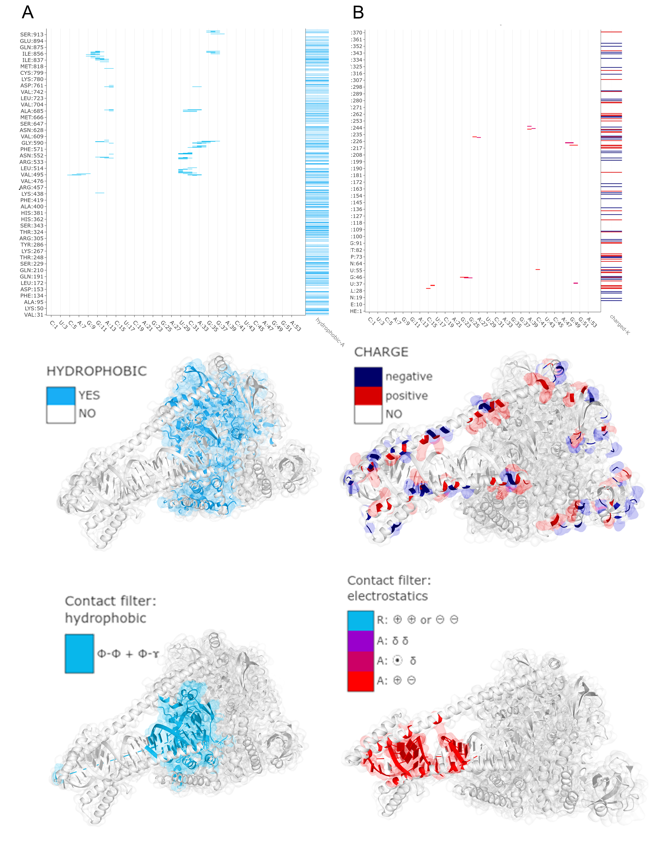
The nsp12 acts as the catalytic unit in the replication of RNA molecules and the catalytic core is composed of conserved hydrophobic regions (Refs: Ahn, D. G., et al. (2012), Kirchdoerfer, R. N., and Andrew B. W (2019)) (see panel A in figure below). The map diagram view was generated by selecting the Hydrophobic option available in Display 1D data along the sequence and setting the Interactive structure coloring to Using 1D features. The hydrophobic contacts between the nsp12 and RNA are visualized using Mapiya by selecting the Hydrophobic option available under Interaction filter and setting the Interactive structure coloring to Using contacts. Two copies of nsp8 bind to opposite sides of the cleft and help in the positioning of the RNA. The long protruding helical extensions in nsp8 contain patches of positively charged regions that act as sliding poles for the exit of RNA (see panel B in figure below), which is essential for the RdRp to process the long genome of SARS-CoV-2 (Ref: Wilamowski, M., et al. (2021)). The non-structural protein 8 (nsp8) helps in the processing of RNA by positioning it in RdRp. The long helical protruding regions in the nsp8 contain patches of positively charged regions that act as sliding poles for the exit of RNA. The sliding poles on the nsp8 are visualized in the interaction map view by selecting the Charged option available in Display 1D data along the sequence and setting the Interactive structure coloring to Using 1D features. The electrostatic interactions are visualized by setting the Electrostatic option available under Interaction filter and setting the Interactive structure coloring to Using contacts.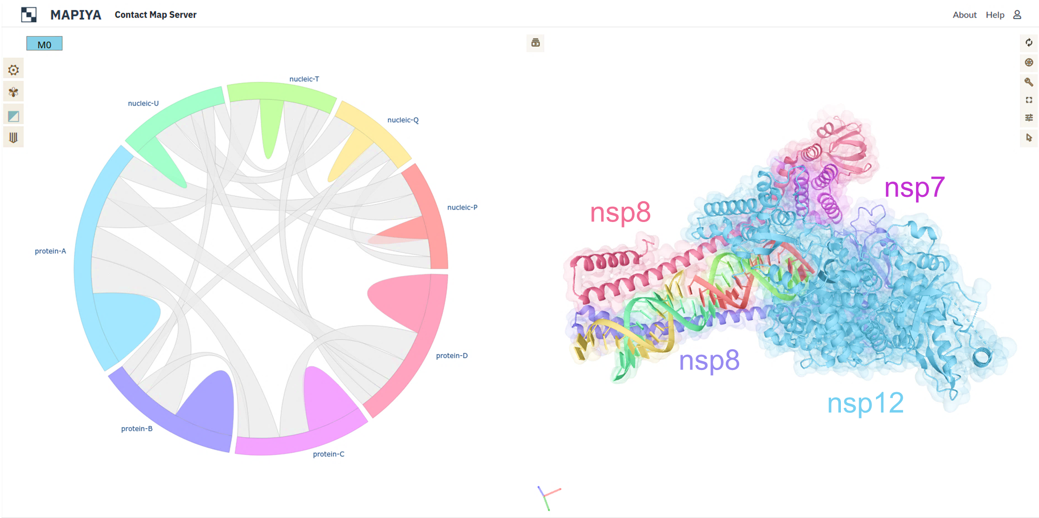
5. Mapiya analysis hints and protocols
Here we provide some additional information on how to better utilize Mapiya.
5.1. Renaming or merging biomolecule chains
The current version of Mapiya was designed to visualize and analyze the interactions between individual biomolecules, separate protein or nucleic acid chains. In some cases, instead of visualizing the interactions between every pair of chains, users may be interested in visualizing the interactions between a set of chains (e.g. double stranded DNA, or a set of protein chains) and another biomolecule. This may be possible by linking the appropriate chains first using external software (also changing the residue numbering may be necessary). Below we provide a python script that may be helpful for that purpose.
https://bitbucket.org/lcbio/mapserver/downloads/rename_chains.py
USAGE:
python rename_chains.py [-h] -f INPUT [-cho CHO] [-chn CHN] [-o OUT]
e.g., python rename_chains.py -f input.pdb -cho A,B -chn C,D -o output.pdb
Options:- -h, print help
- -f, input file in the PDB format (can be multi-model)
- -cho, list of selected chain ids, separated by a comma (e.g., A,B,C) that will be changed
- -chn, list of new chain ids, separated by a comma (e.g., D,D,D)
- -o, name of the output file
- renamepdbchain.pl
- pdb-tools
- GROMACS with command: gmx editconf -f file-in.pdb -o file-out.pdb -resnr [residue number from with to start renumbering] -label [chain id to renumber]